
Alternate Loss Functions for Classification and Robust Regression Can Improve the Accuracy of Artificial Neural Networks
All machine learning algorithms use a loss, cost, utility or reward function to encode the learning objective and oversee the learning process. This function that supervises learning is a frequently unrecognized hyperparameter that determines how incorrect
arxiv.org
개념 설명
인공신경망(ANN, Artificial Neural Network)

인공신경망은 주어진 데이터셋을 근사시키는 함수를 구하는 모델이다. 이러한 모델을 이용하여 새로운 입력값에 대하여 이를 분류(Classification)하거나 결과값을 예측(Regression)하는 등의 Task에 사용된다.
Loss Function (Cost Function)

위와 같은 인공신경망은 데이터셋을 근사시키는 함수를 바로 구할 수 없기 때문에 여러 번에 거쳐 데이터셋에 더 적합한 모델 파라미터들을 구하는 방식으로 데이터셋을 근사시키는 함수를 구한다. 이 과정에서 어떠한 모델의 파라미터들이 더 데이터셋에 적합한지 수치적으로 나타내는 것이 필요한데, 이러한 함수를 손실 함수(Loss Function) 또는 비용 함수(Cost Function)이라고 한다. 이러한 Loss Function은 데이터셋과 모델이 나타내는 근사 함수의 차이를 하나의 스칼라값으로 나타낸다.
Gradient Descent

특별한 경우를 제외하고는 데이터셋을 근사시키는 함수를 바로 구할 수 없다. 데이터셋을 근사시키는 함수를 나타내기 위하여 인공신경망 모델은 매우 많은 가중치(Weight)들과 편향(Bias)값을 이용하는데, 데이터셋을 근사하는 함수를 바로 구하기 위해서는 인공신경망 모델의 모든 가중치(Weight)들과 편향(Bias)값을 닫힌 형태의 해(Closed-form solution)으로 나타낼 수 있어야 한다. 하지만 이는 수학적으로 불가능하다.
이러한 제약 속에서 이를 해결하기 위해 나온 방법이 경사하강법(Gradient Descent)이다. 임의의 가중치와 편향에서 시작하여 Loss Function의 값을 최소화하는 방향으로 가중치와 편향들을 조정하여 Loss Function의 최솟값을 찾아가는 방식이다. 이러한 과정을 진행하기 위하여 Loss Function은 미분가능하여야 한다.
Convexity and Convex Functions

어떠한 함수가 Convex 하다는 것은 함수의 형태가 볼록하다는 것이고, 수학적으로는 함수 위의 임의의 두 점을 연결하는 선을 그래프에 그었을 때, 그 선이 아래 그림과 같이 함수 그래프의 위쪽만을 지나가는 함수를 일컫는다.
Convex한 함수는 Local Minima(지역 최솟값)이 Global Minima(전역 최솟값)과 같다는 것이고, 이는 경사하강법으로 찾은 지역 최솟값이 전역 최솟값과 동일하다는 보장을 하기 때문에 인공 신경망에서 Convex한 Loss Function은 굉장한 이점을 가지게 된다.
0. 개요
회귀(Regression)에는 Loss Function으로써 일반적으로 MSE(Mean Squared Error)가 많이 사용되며, 분류(Classfication)에는 Loss Function으로써 일반적으로 Cross Entropy Loss(CE)가 많이 사용된다.
1. 본문
1.1. Loss Function의 조건과 특성
Loss Function은 다음과 같은 조건을 만족하여야 한다.
- Loss를 나타내어야 한다
1. $\hat{y}=y$일 때 $l(y, \hat{y}) = 0$이어야 한다.
2. $l(0, 0)=l(1, 1)=0$이어야 한다
3. $lim_{\hat{y} \rightarrow 1}l(0,\hat{y})=\infty$, $lim_{\hat{y} \rightarrow 0}l(10,\hat{y})=\infty$이어야 한다 - 미분 가능하여야 한다
경사하강법은 Loss Function을 미분하여 사용하므로 $l(0, \hat{y})$와 $l(1, \hat{y})$은 미분 가능하여야 한다. - Convex한 함수여야 한다
Convex한 Loss Function은 Local Minima와 Global Minima의 동일성을 보장하므로 Convex한 Loss Function은 이점이 있다.
1.2. Loss Function의 비교 - Strictness and Leniency
Strictness (n.) 엄격성
Leniency (n.) 관용성
두 Loss Function을 비교하기 위하여 이 논문에서는 Loss Function의 Strictness를 정의한다
Defininition. 두 Loss Functon $\mathcal{L}_1 (\hat{y}, y)$과 $\mathcal{L} _2 (\hat{y}, y)$에 대하여 어떤 $hat{y}$값들의 집합에 대하여 다음을 만족할 때 $\mathcal{L}_1$이 $\mathcal{L}_2$보다 strict하다고 하자.
$$\frac{\partial \mathcal{L}_1 }{ \partial \hat{y}} \ge \frac{ \partial \mathcal{L}_2}{ \partial \hat{y}}$$
또한 이의 반대 용어인 Leniency를 다음과 같이 정의한다.
Defininition. 두 Loss Functon $\mathcal{L}_1 (\hat{y}, y)$과 $\mathcal{L} _2 (\hat{y}, y)$에 대하여 어떤 $hat{y}$값들의 집합에 대하여 다음을 만족할 때 $\mathcal{L}_1$이 $\mathcal{L}_2$보다 lenient하다고 하자.
$$\frac{\partial \mathcal{L}_1 }{ \partial \hat{y}} \lt \frac{ \partial \mathcal{L}_2}{ \partial \hat{y}}$$
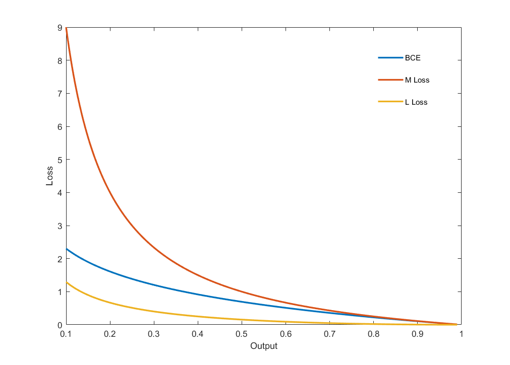
1.3. New Loss Functions - Classification
이 논문에서는 1.1.을 만족하는 Loss FunctIon을 제안한다.
M Loss
$$M(y, \hat{y}) = y \left(\frac{1}{\hat{y} - 1}\right)$$
L Loss
$$L(y, \hat{y}) = \frac{y}{\sqrt{1- (1- \hat{y})^2}} - 1$$
위에 제시한 M Loss와 L Loss는 $y=0$일때만 loss가 0이 되고 $y=1$일 때만 Loss 함수가 동작한다. 아래 Full Loss는 이를 보완해서 제시하였다.
Full M Loss
$$M(y, \hat{y}) = \frac{y}{\hat{y}} + \frac{1-y}{1-\hat{y}} - 1$$
Full L Loss
$$L(y, \hat{y}) = \frac{y}{\sqrt{1- (1- \hat{y})^2}} + \frac{1-y}{\sqrt{1-\hat{y}}} - 1$$
1.4. New Loss Functions - Regression
다양한 Regression Loss Functions (참고)
MAE(Mean Average Error, L2 Error)
$$\mathcal{L}=\frac{1}{N}\sum_{i=1}^{N}{(y_i - \hat{y_i})^2}$$
MSE(Mean Squared Error, L1 Error)
$$\mathcal{L}=\frac{1}{N}\sum_{i=1}^{N}{|y_i - \hat{y_i}|}$$
Huber Loss (Smooth L1 Error)
$$E(y, \hat{y}) = \begin{cases} \frac{1}{2} (y - \hat{y})^2 & \text{for} |y-\hat{y}| \le \delta \\ \delta\left( |y-\hat{y}|- \frac{1}{2}\delta \right) & \text{for} |y-\hat{y}| \gt \delta \end{cases}$$
$$\mathcal{L}=\frac{1}{N}\sum_{i=1}^{N}{E(y_i, \hat{y_i})}$$
Log-Cosh
$$\mathcal{L}=\frac{1}{N}\sum_{i=1}^{N}{\log(\cosh(\hat{y_i} - y_i))}$$
회귀(Regression) 문제에는 MSE(Mean Squared Error)가 자주 이용되는데, MSE는 Outliar(이상치)에 너무 민감하여 MAE(Mean Average Error)의 미분 가능한 버전이 필요한 경우가 많다. MAE(Mean Average Error)가 직접적으로 이용되지 못하는 이유는 다음 2가지 이유가 크다.
- 0에서 미분 불가능하다.
- 0에서 미분값이 커 경사하강법을 진행하면 진동한다.
이 논문에서는 Smooth MAE(SMAE) Loss를 제안한다.
$$\text{SMAE}(e) = e \tanh \left( \frac{e}{2} \right)$$
SMAE Loss는 다음과 같은 특징을 가진다.
- $|e|$가 작을 때 ($|e| \ll 1$) SMAE는 MSE에 가깝다 ($\text{SMAE}(e) = e \tanh \left( \frac{e}{2} \right) \approx \frac{e^2}{2}$이므로)
- $|e|$가 클 때 ($|e| \rightarrow 1$) SMAE는 MAE에 가깝다. ($\text{SMAE}(e) = e \tanh \left( \frac{e}{2} \right) \approx |e|$이므로)

2. 검증
2.1. Simple Linear Regression
다음과 같은 1500개의 데이터를 만들어 제시한 SMAE Loss Function의 성능을 확인하였다.
- $y=2x+3$의 모델에 unit variance Gaussian noise를 더한 데이터 1000개
- 평균 벡터가 $\mu = \begin{bmatrix} 6 \\ -10 \end{bmatrix}$이고 공분산 행렬이 $\Sigma = \begin{bmatrix} 1 & 0.3 \\ -0.3 & 1 \end{bmatrix}$인 2D Gaussian distribution

| Loss Function | Parameter Estimation Error (%) | |
| Slope | Y-intercept | |
| SMAE | 8.73 | 22.6 |
| MSE | 68.2 | 205.82 |
| Log-Cosh | 22.76 | 82.3 |
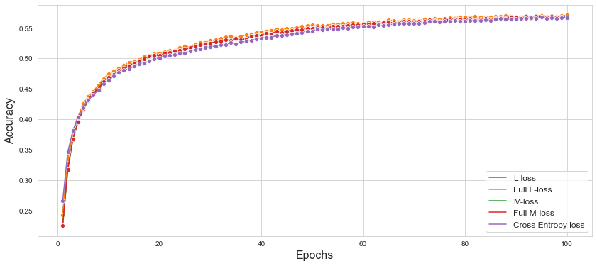
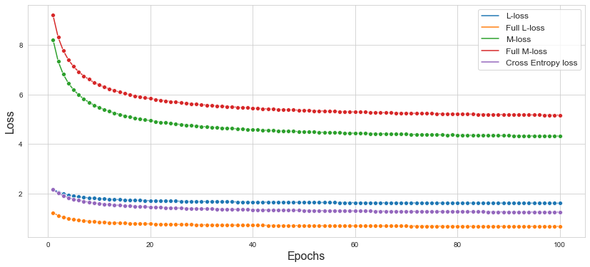
2.2. CIFAR-10
VGG-19 모델의 Loss function을 Cross Entropy Loss, L Loss, M Loss, Full L Loss, Full M Loss를 이용하여 CIFAR-10 데이터셋에 대하여 테스트를 진행하였다.
| Loss Function | Traning Accuracy | Test Accuracy |
| Cross Entropy Loss | 0.5806 | 0.5668 |
| L Loss | 0.5791 | 0.5684 |
| M Loss | 0.5745 | 0.5666 |
| Full L Loss | 0.5827 | 0.5710 |
| Full M Loss | 0.5762 | 0.5668 |
2.3. Imagenette
VGG-19 모델의 Loss function을 Cross Entropy Loss, L Loss, M Loss, Full L Loss, Full M Loss를 이용하여 Imagenette 데이터셋에 대하여 테스트를 진행하였다.
| Loss Function | Traning Accuracy | Test Accuracy |
| Cross Entropy Loss | 0.73 | 0.74 |
| L Loss | 0.75 | 0.77 |
| M Loss | 0.74 | 0.78 |
| Full L Loss | 0.72 | 0.78 |
| Full M Loss | 0.74 | 0.76 |


2.4. Consumer Financial Protection Bureau(CFPB)
LSTM 기반의 모델을 사용하여 Loss function을 Cross Entropy Loss, L Loss, M Loss, Full L Loss, Full M Loss를 이용하여 Consumer Financial Protection Bureau 데이터셋에 대하여 테스트를 진행하였다.
| Loss Function | Traning Accuracy |
| Binary Cross Entropy Loss | 0.822 |
| L Loss | 0.843 |
| M Loss | 0.827 |
| Full L Loss | 0.839 |
| Full M Loss | 0.825 |
2.5. IMDB Movie Review bechmark
BERT 기반의 모델을 사용하여 Loss function을 Cross Entropy Loss, L Loss, M Loss, Full L Loss, Full M Loss를 이용하여 IMDB Movie Review bechmark 데이터셋에 대하여 테스트를 진행하였다.
| Loss Function | Traning Accuracy |
| Binary Cross Entropy Loss | 0.8551 |
| L Loss | 0.8557 |
| M Loss | 0.8539 |
| Full L Loss | 0.8577 |
| Full M Loss | 0.8555 |
3. 결론
BCE Loss보다 Strict하게 정의한 M Loss와 Full M Loss, Binary Cross Entropy Loss보다 Lenient하게 정의한 L Loss와 Full L Loss가 BCE보다 효과적임을 다양한 데이터셋을 통하여 확인할 수 있었으며 이를 통하여 Binary Cross Entropy Loss가 최적의 Loss가 아님을 알 수 있었다. 또한 이로써 Binary Cross Entropy Loss보다 더 좋은 Loss Function이 제시될 수 있음을 보여주었다.
또한 SMAE는 Huber Loss와 같이 추가적인 파라미터를 요구하지 않음에도 Log-Cosh Loss보다 더 Outliar(이상치)에 강함을 확인하였다.


