[2025-1] 주서영 - Flow matching for generative modeling
- ICLR 2023
- 850회 인용
1. Introduction
- 본 논문은 Continuous Normalizaing Flows(CNF)를 시뮬레이션 없이(simulation-free) 효율적으로 훈련할 수 있는 학습 방법인 Flow Matching (FM)을 제시한다.
2. Preliminaries : Continuous Normalizing Flows

- Normalizaing Flow : 데이터 분포인 $x$에서 $z$로의 역변환이 가능한 Flow를 학습하는 모델
- Continuous Normalizing Flows(CNF) : 시간에 따른 vector filed를 학습하여 ODE를 통해 확률 분포를 변환하는 생성 모델
- $\mathbb{R}^d$
- 데이터 포인트 $x=(x^1,\cdots,x^d)\in\mathbb{R}^d$
- Probability Density Path $p_t(x)$
- $p:[0,1]\times{}\mathbb{R}^d\rightarrow{}\mathbb{R}_{>0}$
- probability density path는 데이터가 움직이는 궤적을 말한다. noise 분포를 $t=0$에 두고 data distribution을 $t=1$로 했을 때 noise 분포에서 데이터의 분포까지 옮겨가는 경로를 나타낸다.

- Flow $x_t=\phi_t(x_0)$
- $\phi:[0,1]\times\mathbb{R}^d\rightarrow\mathbb{R}^d$
- $t$시점에 벡터가 어디에 위치할 것인지 결정하는 함수
- Vector Filed $v_t$
- $v:[0,1]\times{}\mathbb{R}^d\rightarrow\mathbb{R}^d$
- $v_t(\phi_t(x_0))=\frac{d}{dt}\phi_t(x_0)$
- Flow $\phi_t$를 미분하는 방정식으로 정의됨 ⇒ ODE
- $t$가 변할 때 vector $\phi_t$가 어디로 향할 것인지를 나타내는 함수
$$
\frac{d}{dt} \phi_t(x) = v_t(\phi_t(x)) \\ \phi_0(x) = x
$$ - 적분 식은 아래와 같으며 $t$시점의 변화를 알 수 있음
$$
\phi_t(x) = \phi_0(x) + \int_0^t v_{\tau} (\phi_{\tau}(x)) d\tau
$$
(2) Push-Forward Equation
- 단순한 데이터 분포를 복잡한 분포로 변환하는 과정
- CNF는 간단한 prior distribution (e.g. : gaussian) $p_0$를 복잡한 분포 $p_1$으로 변환하는 것을 가능하게 함
- push-forward equation을 사용하여 $p_1$이 모델링해야 하는 데이터 분포 $q$에 가깝도록 만들도록 함
$$
p_t = [ \phi_t ]* p_0\\\forall x \in \mathbb{R}^2, \quad [\phi_t]* p_0(x) = p_0(\phi_t^{-1}(x)) \det \left[ \frac{\partial \phi_t^{-1}}{\partial x}(x) \right]
$$
- $\phi_t$ : 하나의 파라미터화된 모델
⇒ $v_t$가 praobability path $p_t$를 생성하게 됨
3. Flow Matching
(1) Flow Matching
- $p_t$ : probability density path로 t에 따라 확률 분포가 어떻게 변하는지
- $v_t$ : neural network의 output
- $u_t$ : true vector field
⇒ neural network output인 $v_t$와 정답이 되는 vector field $u_t$를 매칭시키는 것을 목표로 함
$$
\mathcal{L}{FM}(\theta) = \mathbb{E}_{t, p_t(x)} || v_t(x) - u_t(x) ||^2
$$
- target인 true vector filed인 $u_t(x)$에 대한 정보가 부족함 (intractable)
⇒ vector field $u_t(x)$ 대신에 conditional vector field인 $u_t(x_t|x_1)$을 고려
(2) Conditional Flow Matching
Conditional Flow Matching은 Flow matching의 목표와 동일한 최적화를 제공하면서 계산 복잡성을 줄이고 실용적으로 사용할 수 있는 접근 방법이다.
$where\quad{}x_1 \sim q(x_1) \approx p_1(x_1)$
$$
\mathcal{L}{CFM}(\theta) = \mathbb{E}_{t, q(x_1), p_t(x|x_1)} || v_t(x) - u_t(x|x_1) ||^2
$$
- $x_1\sim{}q(x_1)$ : $x_1$이 진짜 데이터 분포인 $q(x_1)$에서 샘플링됨
- $p_1(x_1)\approx{}q(x_1)$ : 모델이 학습한 분포 $p_1(x_1)$이 실제 데이터 분포 $q(x_1)$와 가깝도록 만드는 것을 목표로 함
$$
\frac{\partial}{\partial \theta} \left( \mathcal{L}{FM}(\theta) - \mathcal{L}{CFM}(\theta) \right) = 0
$$
- FM objective와 CFM objective를 미분한 것이 같은데 이는 둘의 최적화 과정이 동일하다고 볼 수 있음
4. Conditional Probability Paths and Vector Fileds
intractable한 flow에서 tractable하게 바꾸기 위해 conditional flow 정의에서 conditional path를 구체화 시킴
⇒ $u_t(x_t|x_1)$ 를 구하는 법
(1) Probability Density Path $p_t(x)$
$$
p: [0,1] \times \mathbb{R}^d \to \mathbb{R}_{>0}\\p_t(x | x_1) = \mathcal{N} \left( x \mid \mu_t(x_1), \sigma_t(x_1)^2 I \right)
\\p_0(x) = \mathcal{N} (x \mid 0, I)
$$
$x_1$에 대한 mean과 variance로 normal distribution으로 가정하고 nosie distribution인 $p_0$가 standard normal distribution인 경우 Flow를 구할 수 있음
(2) Flow $\psi_t(x)$
$$
\psi: [0,1] \times \mathbb{R}^d \to \mathbb{R}^d
\
\psi_t(x_0) = \sigma_t(x_1) x_0 + \mu_t(x_1)
$$
(3) Vector Field $u_t$
$$
u: [0,1] \times \mathbb{R}^d \to \mathbb{R}^d\\
u_t(x_t | x_1) = \frac{d}{dt} \psi_t(x_0)
\\= \frac{d}{dt} \psi_t(\psi_t^{-1}(x_t))
\\= \frac{\sigma_t'(x_1)}{\sigma_t(x_1)} (x_t - \mu_t(x_1)) + \mu_t'(x_1)
\\
\therefore \frac{d}{dt} \psi_t(x_0) = \sigma_t'(x_1) x_0 + \mu_t'(x_1)
\\
\psi_t^{-1}(x_t) = \frac{x_t - \mu_t(x_1)}{\sigma_t(x_1)}
$$
- vector filed $u_t$는 $\psi_t$에 대한 미분이며 $x_t$로 식을 바꾸기 위해 inverse를 취함
- $\psi_t$에 대한 미분과 $\psi_t$의 inverse는 Flow 정의에 의해 구할 수 있으며 vector filed $u_t(x_t|x_1)$을 구할 수 있게 됨
(4) Model에서의 Vector Field
① Score-based Model
- Probability Density Path : $\mathcal{N} (x | x_1, \sigma_{(1-t)}^2 I)$
- Flow : $\sigma_{1-t} x_0 + x_1$
- Vector Field : $\frac{\sigma'{1-t}}{\sigma{1-t}} (x_t - x_1)$
② Diffusion Model
- Probability Density Path : $\mathcal{N} (x | \alpha_{1-t} x_1, (1 - \alpha_{1-t}^2) I)$
- Flow : $\sqrt{1 - \alpha_{1-t}^2} x_0 + \alpha_{1-t} x_1$
- Vector Field : $\frac{\alpha'{1-t}}{1 - \alpha{1-t}^2} (\alpha_{1-t} x_t - x_1)$
③ Optimal Transport
- Probability Density Path : $\mathcal{N} (x | t x_1, (1 - (1 - \sigma_{\min}) t)^2 I)$
- Flow : $(1 - (1 - \sigma_{\min}) t) x_0 + t x_1$
- Vector Field : $\frac{x_1 - (1 - \sigma_{\min}) x_t}{1 - (1 - \sigma_{\min}) t}$
⇒ probability density patu에서 $t=0$이면 noise이고 $t=1$이면 data distribution이 됨
⇒ Flow는 $x_0$와 $x_1$이 linear interpolation하는 지점
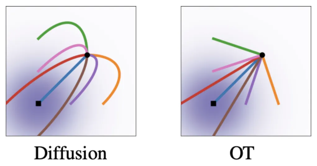
- vector filed를 그렸을 때 Diffusion에서 곡선 형태, OT는 직선 형태의 모습을 관찰할 수 있으며 OT가 data distribution을 짧은 시간에 도달하는 것을 알 수 있음
5. Experiments

- Gaussian Path이기 때문에 Flow mathcing을 활용해서 diffusion에 적용할 수 있음
- FM Diffusion을 살펴보면 diffusion에서 flow mathcing을 적용하면 성능이 좋아진 것을 볼 수 있음

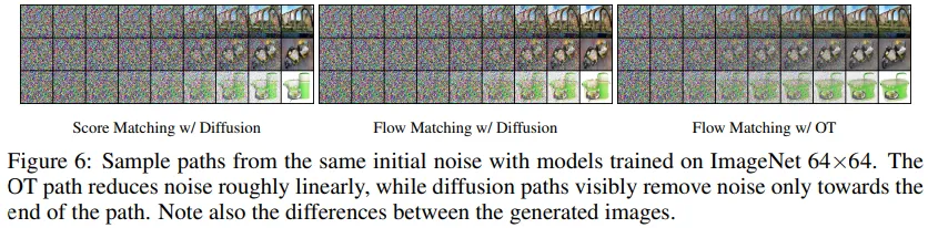
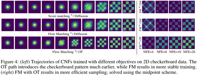
- Flow Mathing과 OT(Optimal Transport)를 적용했을 때 이미지가 빨리 생성되는 것을 볼 수 있음
6. Conclusion
- Flow Matching은 Continuous Normalizaing Flows의 안정적이고 더 빠른 학습이 가능하게 함
[참고]
https://velog.io/@guts4/FLOW-MATCHING-FOR-GENERATIVE-MODELING
https://mlg.eng.cam.ac.uk/blog/2024/01/20/flow-matching.html#normalising-flows
https://lilianweng.github.io/posts/2021-07-11-diffusion-models/
https://www.youtube.com/watch?v=YFZbFr3cjpA
https://www.youtube.com/watch?v=9zauDLVrKJg